Graphics Math #1: 2D Transformations
I am going to help demystify how math is used for computer graphics. We’ll start simple by looking at 2D transformations.
What we learn about using matrices for 2D transformations will become applicable to 3D – it just involves slightly larger matrices and a few more operations to make the leap from 2D to 3D. 2D is simpler to visualize and understand, so that is where our introduction will begin.
Although we will be using matrices and vectors, you will not need a deep understanding of linear algebra to follow this article. The math will be explained along the way to help you get a better understanding of how it is being applied to 2D graphics transformations.
What is Linear Algebra?
Linear algebra is a branch of math that involves systems of linear equations. A linear equation is simply an equation that describes a straight line. You likely learned a form of a line equation that looks like \(y = mx + b\), but the form used in linear algebra looks more like \(ax + by = c\). Converting from one form to another is just doing a little algebra, so \(y = mx + b \) is the same as \(-mx + 1y = b\) after moving the \(x\) over to the other side.
A system of linear equations is just multiple related linear equations describing multiple straight lines. Solving a system of linear equations will find the values of unknowns \((x, y, z)\) that can make all of the equations equal their respective corresponding value – finding the point where all of these lines cross.
$$ \begin{aligned} c_{1}x + c_{2}y + c_{3}z &= v_{1} \\ c_{4}x + c_{5}y + c_{6}z &= v_{2} \\ c_{7}x + c_{8}y + c_{9}z &= v_{3} \end{aligned} $$We are not going to be solving systems of linear equations in this article. Instead, we will be using matrices to represent the values of these coefficients and use matrix multiplication to get the results of applying it to a known point to get a resulting transformed point. The above linear equations and the matrix multiplication below are equivalent, but use different notation.
$$ \begin{bmatrix} c_{1} & c_{2} & c_{3} \\ c_{4} & c_{5} & c_{6} \\ c_{7} & c_{8} & c_{9} \end{bmatrix} \times \begin{bmatrix} x \\ y \\ z \end{bmatrix} = \begin{bmatrix} v_{1} \\ v_{2} \\ v_{3} \end{bmatrix} $$Matrix multiplication is extremely useful in computer graphics because it can be used to “apply” multiple transformations to get a resulting transformation matrix that can be used to move points. The main transformations we will be concerned with are translation (moving points along the \(x\) and \(y\) axes), rotation (pivoting points around the center origin \((0, 0)\)), and scaling (moving points farther or closer to the origin, or growing and shrinking the graphics). There is also shearing (skewing an object to be tilted), but that isn’t used as often in games as the other transformations.
You may be asking yourself, “How the heck does a box full of numbers do all that?” Hopefully this illustration can help you visualize it. Imagine a sheet of graph paper. Each square is one unit by one unit in size. Let the center of the graph paper to be the “origin” with a cartesian coordinate of \((0, 0)\). The \(x\) axis points to the right and the \(y\) axis points up. Let’s put a dot at the coordinate \((2, 3)\).
Now imagine rotating the sheet of paper on your desk, so now the \(x\) axis is pointing at an angle up and to the right and the \(y\) axis is now pointing up and to the left. The dot is still at coordinate \((2, 3)\), but because the graph paper had been rotated, that coordinate looks like it is now in a different place. You can think of these matrix transformations as being like moving, rotating, and changing the size of the graph paper and that has an effect on where coordinates on the graph paper appear to be. The dot appeared to have moved, but really the space the dot’s coordinates are in is what had changed.
You can imagine how these can be combined to move an object around the screen – it could be first scaled to make it larger, then rotated to face a different direction, and then translated to move the object to a different place on the screen. Any number of transformations can be applied in any order by multiplying each of their matrices together and result is a matrix that describes the end result after all this manipulation.
Subscript Notation
To understand how matrix/vector and matrix/matrix multiplication is performed, I want to ensure you understand subscript notation for referencing elements in the matrices and vectors. It is similar to array indexes in computer programming. You can see in this small example how a row and column are referred to by using a subscript (small text that is slightly lower):
$$ M = \begin{bmatrix} 1 & 2 & 3 \\ 4 & 5 & 6 \\ 7 & 8 & 9 \end{bmatrix} $$$$ \begin{aligned} M_{\text{row column}} &= \text{value} \\ M_{12} &= 2 \\ M_{31} &= 7 \end{aligned} $$Transforming a 2D Point
Transforming a point is done by multiplying the vertex position vector by a transformation matrix. This is what multiplying a row major layout matrix with column vectors looks like.
$$ \begin{bmatrix} m_{11} & m_{12} & m_{13} \\ m_{21} & m_{22} & m_{23} \\ m_{31} & m_{32} & m_{33} \end{bmatrix} \times \begin{bmatrix} x \\ y \\ z \end{bmatrix} = \begin{bmatrix} m_{11}x + m_{12}y + m_{13}z \\ m_{21}x + m_{22}y + m_{23}z \\ m_{31}x + m_{32}y + m_{33}z \end{bmatrix} $$Since we are using affine transformations (preserving parallel lines), the bottom row of our matrix stays \([0, 0, 1]\), so we can write it this way and only care about the top two result values for our transformed point coordinate:
$$ \begin{bmatrix} m_{11} & m_{12} & m_{13} \\ m_{21} & m_{22} & m_{23} \\ 0 & 0 & 1 \end{bmatrix} \times \begin{bmatrix} x \\ y \\ 1 \end{bmatrix} = \begin{bmatrix} m_{11}x + m_{12}y + m_{13} \\ m_{21}x + m_{22}y + m_{23} \\ 1 \end{bmatrix} $$What Matrices Will We Use?
Even though 2D points only have an \(x\) and \(y\) coordinate, we will be using \(3 \times 3\) matrices for our 2D graphics transformations. Why not use a \(2 \times 2\) matrix? We could, if all we cared about was rotation and scaling, but we also want to be able to translate objects in our 2D scene. The extra row and column let us do that. For the same reason, with 3D graphics a \(4 \times 4\) matrix is used.
Identity Matrix
The simplest matrix to understand is the “Identity Matrix”. It is a matrix that basically does nothing – a vertex “transformed” by it will stay exactly the same. It is simply constructed with ones along the diagonal and the rest filled in with zeros.
$$ \begin{bmatrix} 1 & 0 & 0 \\ 0 & 1 & 0 \\ 0 & 0 & 1 \end{bmatrix} $$If we look at the system of linear equations representation, it is easier to get an intuition about how it works. The ones keep the variables that correspond to the row, and the zeros remove the variables we don’t need. This leaves only one variable for each vector element – the same as it was before.
$$ \begin{aligned} 1x + 0y + 0z &= x \\ 0x + 1y + 0z &= y \\ 0x + 0y + 1z &= z \end{aligned} $$Since this doesn’t actually do anything, we won’t likely need to use it in a graphics program. This was provided as the simplest example “transformation” we could do.
2D Scale
The next simplest transformation is scaling. Instead of just ones along the diagonal, we can have a scaling factor correspond to the \(x\) and \(y\) vector components. Multiplying them by a scaling factor makes an object look like it is growing or shrinking by moving vertices either farther away or closer to the origin.
$$ \begin{bmatrix} s_x & 0 & 0 \\ 0 & s_y & 0 \\ 0 & 0 & 1 \end{bmatrix} $$Which results in these equations when a vector is multiplied by it:
$$ \begin{aligned} s_x x + 0y + 0z &= s_x x \\ 0x + s_y y + 0z &= s_y y \\ 0x + 0y + 1z &= z \end{aligned} $$2D Translation
Translating a 2D point is simply adding some amount to move the vertex horizontally and/or vertically.
$$ \begin{bmatrix} 1 & 0 & t_x \\ 0 & 1 & t_y \\ 0 & 0 & 1 \end{bmatrix} $$Which looks like these equations when applied:
$$ \begin{aligned} 1x + 0y + t_x z &= x + t_x z \\ 0x + 1y + t_y z &= y + t_y z \\ 0x + 0y + 1z &= z \end{aligned} $$It would be a good time to mention that the vectors we are using have \(x\) and \(y\) for the horizontal and vertical position of the vertex, but the vector is three elements in size. We will always use \(1\) for the third \((z)\) component. This makes things simpler to see – since \(z\) is always one, what gets added is the amount to translate the coordinate by.
$$ \begin{aligned} 1x + 0y + t_x(1) &= x + t_x \\ 0x + 1y + t_y(1) &= y + t_y \\ 0x + 0y + 1(1) &= 1 \end{aligned} $$2D Shearing
Horizontal shearing changes the value of \(x\) as \(y\) changes. For example, the higher on the screen a point is, the more right it might also be moved. This causes the grid of the world’s “graph paper” to be made from parallelograms instead of squares.
$$ \begin{bmatrix} 1 & s_x & 0 \\ 0 & 1 & 0 \\ 0 & 0 & 1 \end{bmatrix} $$You can see in the linear equation form when applied to a vector that the value of the transformed \(x\) is also changing with the value of \(y\).
$$ \begin{aligned} 1x + s_x y + 0z &= x + s_x y \\ 0x + 1y + 0z &= y \\ 0x + 0y + 1z &= z \end{aligned} $$Vertical shearing is essentially the same as horizontal shearing, but along the other axis.
$$ \begin{bmatrix} 1 & 0 & 0 \\ s_y & 1 & 0 \\ 0 & 0 & 1 \end{bmatrix} $$Which looks like this:
$$ \begin{aligned} 1x + 0 y + 0z &= x \\ s_y x + 1y + 0z &= s_y x + y \\ 0x + 0y + 1z &= z \end{aligned} $$2D Rotation
Rotation is performed in a counter-clockwise turn, with the common convention of zero degrees being pointing right along the positive \(x\) axis. This is the 2D rotation transformation matrix, where sine and cosine are used to rotate points along a circular path. Sine and cosine correspond to points on a unit circle at a given amount of rotation.
$$ \begin{bmatrix} \cos\theta & -\sin\theta & 0 \\ \sin\theta & \cos\theta & 0 \\ 0 & 0 & 1 \end{bmatrix} $$Initially, it might not seem obvious why the first row has a negative sine, but the second row does not negate sine. Let’s consider a concrete example to see why. Consider a point that is starting at (3, 1) and will be rotated counter-clockwise by 90 degrees to end up at (-1, 3).
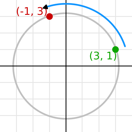
When the angle \(\theta\) is \(0^\circ\), no rotation is performed because \(sin 0^\circ = 0\) and \(cos 0^\circ = 1\), so it resembles the identity matrix:
$$ \begin{bmatrix} 1 & 0 & 0 \\ 0 & 1 & 0 \\ 0 & 0 & 1 \end{bmatrix} $$When the angle \(\theta\) is \(90^\circ\), a quarter rotation is made counter-clockwise. Since \(\sin 90^\circ = 1\) and \(\cos 90^\circ = 0\), we get a matrix that looks like this:
$$ \begin{bmatrix} 0 & -1 & 0 \\ 1 & 0 & 0 \\ 0 & 0 & 1 \end{bmatrix} $$If we plug in the starting coordinate of \((3, 1)\) for \((x, y)\) into the linear equation that results from multiplying the point’s vector by the rotation matrix, we can see that the resulting transformed new coordinate is \((-1, 3)\) – what we see in the illustration above. Whenever a \(90^\circ\) rotation is made, a sign needs to flip because the point will cross an axis.
$$ \begin{aligned} 0(3) + -1(1) + 0(1) &= -1 \\ 1(3) + 0(1) + 0(1) &= 3 \\ 0(3) + 0(1) + 1(1) &= 1 \end{aligned} $$In the examples I gave, degrees were used. The sin and cos functions available in a programming language most likely use radians – a unit where one radian is the angle at which the arc length equals the radius. These can easily be converted, because a full rotation in radians is \(2\pi\) and a full rotation in degrees is \(360^\circ\).
3×3 Matrix Multiplication Process Illustrated
I will only briefly go over the basic process of multiplying two 3x3 matrices because that is what we are using for 2D graphics – I recommend doing additional research to get a more complete understanding of it. The two 3x3 matrices multiplied together produce a new 3x3 matrix with the results.
To get this resulting matrix, follow this pseudocode’s steps:
For each row in matrix A:
    For each column in matrix B:
        Sum results of:
            For i in length of row and column:
                Get the ith element from the current row.
                Get the ith element from the current column.
                Multiply the row element and column element together.
        Store the sum at position [row, column] in the result matrix.
The full process of performing this procedure on the full matrix will look like this:
Step 1: Row 1 of A × Column 1 of B → entry \(c_{11}\)
$$ \begin{bmatrix} \textcolor{blue}{a_{11}} & \textcolor{blue}{a_{12}} & \textcolor{blue}{a_{13}} \\ a_{21} & a_{22} & a_{23} \\ a_{31} & a_{32} & a_{33} \end{bmatrix} \times \begin{bmatrix} \textcolor{red}{b_{11}} & b_{12} & b_{13} \\ \textcolor{red}{b_{21}} & b_{22} & b_{23} \\ \textcolor{red}{b_{31}} & b_{32} & b_{33} \end{bmatrix} = \begin{bmatrix} \textcolor{blue}{a_{11}}\textcolor{red}{b_{11}} + \textcolor{blue}{a_{12}}\textcolor{red}{b_{21}} + \textcolor{blue}{a_{13}}\textcolor{red}{b_{31}} & \cdot & \cdot \\ \cdot & \cdot & \cdot \\ \cdot & \cdot & \cdot \end{bmatrix} $$Step 2: Row 1 of A × Column 2 of B → entry \(c_{12}\)
$$ \begin{bmatrix} \textcolor{blue}{a_{11}} & \textcolor{blue}{a_{12}} & \textcolor{blue}{a_{13}} \\ a_{21} & a_{22} & a_{23} \\ a_{31} & a_{32} & a_{33} \end{bmatrix} \times \begin{bmatrix} b_{11} & \textcolor{red}{b_{12}} & b_{13} \\ b_{21} & \textcolor{red}{b_{22}} & b_{23} \\ b_{31} & \textcolor{red}{b_{32}} & b_{33} \end{bmatrix} = \begin{bmatrix} c_{11} & \textcolor{blue}{a_{11}}\textcolor{red}{b_{12}} + \textcolor{blue}{a_{12}}\textcolor{red}{b_{22}} + \textcolor{blue}{a_{13}}\textcolor{red}{b_{32}} & \cdot \\ \cdot & \cdot & \cdot \\ \cdot & \cdot & \cdot \end{bmatrix} $$Step 3: Row 1 of A × Column 3 of B → entry \(c_{13}\)
$$ \begin{bmatrix} \textcolor{blue}{a_{11}} & \textcolor{blue}{a_{12}} & \textcolor{blue}{a_{13}} \\ a_{21} & a_{22} & a_{23} \\ a_{31} & a_{32} & a_{33} \end{bmatrix} \times \begin{bmatrix} b_{11} & b_{12} & \textcolor{red}{b_{13}} \\ b_{21} & b_{22} & \textcolor{red}{b_{23}} \\ b_{31} & b_{32} & \textcolor{red}{b_{33}} \end{bmatrix} = \begin{bmatrix} c_{11} & c_{12} & \textcolor{blue}{a_{11}}\textcolor{red}{b_{13}} + \textcolor{blue}{a_{12}}\textcolor{red}{b_{23}} + \textcolor{blue}{a_{13}}\textcolor{red}{b_{33}} \\ \cdot & \cdot & \cdot \\ \cdot & \cdot & \cdot \end{bmatrix} $$Step 4: Row 2 of A × Column 1 of B → entry \(c_{21}\)
$$ \begin{bmatrix} a_{11} & a_{12} & a_{13} \\ \textcolor{blue}{a_{21}} & \textcolor{blue}{a_{22}} & \textcolor{blue}{a_{23}} \\ a_{31} & a_{32} & a_{33} \end{bmatrix} \times \begin{bmatrix} \textcolor{red}{b_{11}} & b_{12} & b_{13} \\ \textcolor{red}{b_{21}} & b_{22} & b_{23} \\ \textcolor{red}{b_{31}} & b_{32} & b_{33} \end{bmatrix} = \begin{bmatrix} c_{11} & c_{12} & c_{13} \\ \textcolor{blue}{a_{21}}\textcolor{red}{b_{11}} + \textcolor{blue}{a_{22}}\textcolor{red}{b_{21}} + \textcolor{blue}{a_{23}}\textcolor{red}{b_{31}} & \cdot & \cdot \\ \cdot & \cdot & \cdot \end{bmatrix} $$Step 5: Row 2 of A × Column 2 of B → entry \(c_{22}\)
$$ \begin{bmatrix} a_{11} & a_{12} & a_{13} \\ \textcolor{blue}{a_{21}} & \textcolor{blue}{a_{22}} & \textcolor{blue}{a_{23}} \\ a_{31} & a_{32} & a_{33} \end{bmatrix} \times \begin{bmatrix} b_{11} & \textcolor{red}{b_{12}} & b_{13} \\ b_{21} & \textcolor{red}{b_{22}} & b_{23} \\ b_{31} & \textcolor{red}{b_{32}} & b_{33} \end{bmatrix} = \begin{bmatrix} c_{11} & c_{12} & c_{13} \\ c_{21} & \textcolor{blue}{a_{21}}\textcolor{red}{b_{12}} + \textcolor{blue}{a_{22}}\textcolor{red}{b_{22}} + \textcolor{blue}{a_{23}}\textcolor{red}{b_{32}} & \cdot \\ \cdot & \cdot & \cdot \end{bmatrix} $$Step 6: Row 2 of A × Column 3 of B → entry \(c_{23}\)
$$ \begin{bmatrix} a_{11} & a_{12} & a_{13} \\ \textcolor{blue}{a_{21}} & \textcolor{blue}{a_{22}} & \textcolor{blue}{a_{23}} \\ a_{31} & a_{32} & a_{33} \end{bmatrix} \times \begin{bmatrix} b_{11} & b_{12} & \textcolor{red}{b_{13}} \\ b_{21} & b_{22} & \textcolor{red}{b_{23}} \\ b_{31} & b_{32} & \textcolor{red}{b_{33}} \end{bmatrix} = \begin{bmatrix} c_{11} & c_{12} & c_{13} \\ c_{21} & c_{22} & \textcolor{blue}{a_{21}}\textcolor{red}{b_{13}} + \textcolor{blue}{a_{22}}\textcolor{red}{b_{23}} + \textcolor{blue}{a_{23}}\textcolor{red}{b_{33}} \\ \cdot & \cdot & \cdot \end{bmatrix} $$Step 7: Row 3 of A × Column 1 of B → entry \(c_{31}\)
$$ \begin{bmatrix} a_{11} & a_{12} & a_{13} \\ a_{21} & a_{22} & a_{23} \\ \textcolor{blue}{a_{31}} & \textcolor{blue}{a_{32}} & \textcolor{blue}{a_{33}} \end{bmatrix} \times \begin{bmatrix} \textcolor{red}{b_{11}} & b_{12} & b_{13} \\ \textcolor{red}{b_{21}} & b_{22} & b_{23} \\ \textcolor{red}{b_{31}} & b_{32} & b_{33} \end{bmatrix} = \begin{bmatrix} c_{11} & c_{12} & c_{13} \\ c_{21} & c_{22} & c_{23} \\ \textcolor{blue}{a_{31}}\textcolor{red}{b_{11}} + \textcolor{blue}{a_{32}}\textcolor{red}{b_{21}} + \textcolor{blue}{a_{33}}\textcolor{red}{b_{31}} & \cdot & \cdot \end{bmatrix} $$Step 8: Row 3 of A × Column 2 of B → entry \(c_{32}\)
$$ \begin{bmatrix} a_{11} & a_{12} & a_{13} \\ a_{21} & a_{22} & a_{23} \\ \textcolor{blue}{a_{31}} & \textcolor{blue}{a_{32}} & \textcolor{blue}{a_{33}} \end{bmatrix} \times \begin{bmatrix} b_{11} & \textcolor{red}{b_{12}} & b_{13} \\ b_{21} & \textcolor{red}{b_{22}} & b_{23} \\ b_{31} & \textcolor{red}{b_{32}} & b_{33} \end{bmatrix} = \begin{bmatrix} c_{11} & c_{12} & c_{13} \\ c_{21} & c_{22} & c_{23} \\ c_{31} & \textcolor{blue}{a_{31}}\textcolor{red}{b_{12}} + \textcolor{blue}{a_{32}}\textcolor{red}{b_{22}} + \textcolor{blue}{a_{33}}\textcolor{red}{b_{32}} & \cdot \end{bmatrix} $$Step 9: Row 3 of A × Column 3 of B → entry \(c_{33}\)
$$ \begin{bmatrix} a_{11} & a_{12} & a_{13} \\ a_{21} & a_{22} & a_{23} \\ \textcolor{blue}{a_{31}} & \textcolor{blue}{a_{32}} & \textcolor{blue}{a_{33}} \end{bmatrix} \times \begin{bmatrix} b_{11} & b_{12} & \textcolor{red}{b_{13}} \\ b_{21} & b_{22} & \textcolor{red}{b_{23}} \\ b_{31} & b_{32} & \textcolor{red}{b_{33}} \end{bmatrix} = \begin{bmatrix} c_{11} & c_{12} & c_{13} \\ c_{21} & c_{22} & c_{23} \\ c_{31} & c_{32} & \textcolor{blue}{a_{31}}\textcolor{red}{b_{13}} + \textcolor{blue}{a_{32}}\textcolor{red}{b_{23}} + \textcolor{blue}{a_{33}}\textcolor{red}{b_{33}} \end{bmatrix} $$Final: Full result
$$ \begin{bmatrix} a_{11} & a_{12} & a_{13} \\ a_{21} & a_{22} & a_{23} \\ a_{31} & a_{32} & a_{33} \end{bmatrix} \times \begin{bmatrix} b_{11} & b_{12} & b_{13} \\ b_{21} & b_{22} & b_{23} \\ b_{31} & b_{32} & b_{33} \end{bmatrix} = $$$$ \begin{bmatrix} a_{11}b_{11}+a_{12}b_{21}+a_{13}b_{31} & a_{11}b_{12}+a_{12}b_{22}+a_{13}b_{32} & a_{11}b_{13}+a_{12}b_{23}+a_{13}b_{33} \\ a_{21}b_{11}+a_{22}b_{21}+a_{23}b_{31} & a_{21}b_{12}+a_{22}b_{22}+a_{23}b_{32} & a_{21}b_{13}+a_{22}b_{23}+a_{23}b_{33} \\ a_{31}b_{11}+a_{32}b_{21}+a_{33}b_{31} & a_{31}b_{12}+a_{32}b_{22}+a_{33}b_{32} & a_{31}b_{13}+a_{32}b_{23}+a_{33}b_{33} \end{bmatrix} $$Order Matters
The final thing to make clear is that the order of matrix multiplication matters. Usually these matrices are multiplied to first scale, then rotate, then translate. A clear example is to consider the result of rotating then translating vs. translating then rotating. If you rotate an object 90 degrees (turning it from facing right to now face up) then translate left ten units, the object will be at \((-10, 0)\) and facing up. If you do it the other way around and translate first, the rotating will swing it around like it is on the end of a stick and the object will instead be at \((0, -10)\).
Multiplication is applied from right to left, so if you had a vector \(v\), a translation matrix \(T\), a rotation matrix \(R\), and a scale matrix \(S\), it would be written out in this order:
$$ v' = T \times R \times S \times v $$What Might Be Covered Later
This just scratches the surface of graphics programming, but it is enough to get started with writing a program that moves shapes around the screen. Possible topics for future articles include the model/view/projection matrices, going into the 3rd dimension, or affine texture mapping. Keep an eye out for if these articles get written.